An end-to-end differentiable depth imaging system which jointly optimizes the LiDAR scanning pattern and sparse depth inpainting.

Abstract

Current LiDAR systems are limited in their ability to capture dense 3D point clouds. To overcome this challenge, deep learning-based depth completion algorithms have been developed to inpaint missing depth guided by an RGB image. However, these methods fail for low sampling rates. Here, we propose an adaptive sampling scheme for LiDAR systems that demonstrates state-of-the-art performance for depth completion at low sampling rates. Our system is fully differentiable, allowing the sparse depth sampling and the depth inpainting components to be trained end-to-end with an upstream task.

Network Model

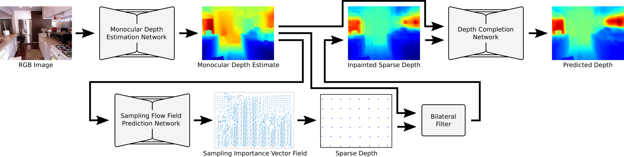
The deep adaptive LiDAR model takes as input an RGB image and predicts an optimal sampling pattern and reconstructed dense depth from sampling at these locations. A pre-trained monocular depth estimation network is used to make an initial estimate of depth in the scene. A U-Net is used to extract a sampling importance vector field, which is then integrated and used for sampling from the scene. Another U-Net is used to fuse the coarsely inpainted sparse depth samples with the monocular depth estimate in order to predict the dense depth.

Adaptive Sampling

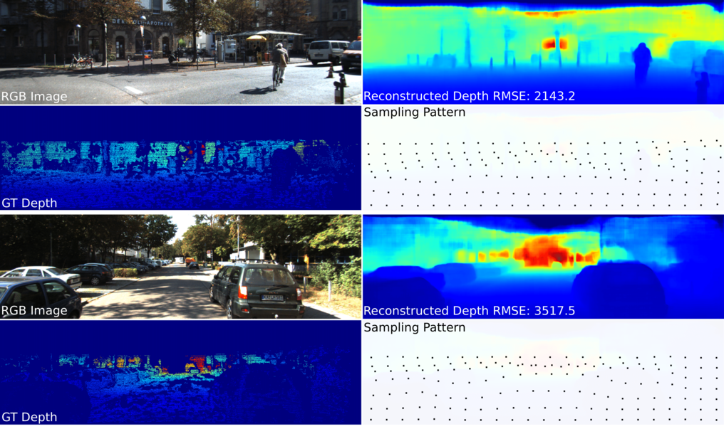
Optimal sampling patterns: Depth estimations and predicted sparse sampling patterns for the KITTI validation dataset. The left column contains RGB image and ground truth depth measurements, and the right column contains the reconstructed depth images and the predicted sparse sampling patterns in order to reconstruct those depth images. RMSE is measured in millimeters.

Depth Completion

NYU-v2 and KITTI Examples

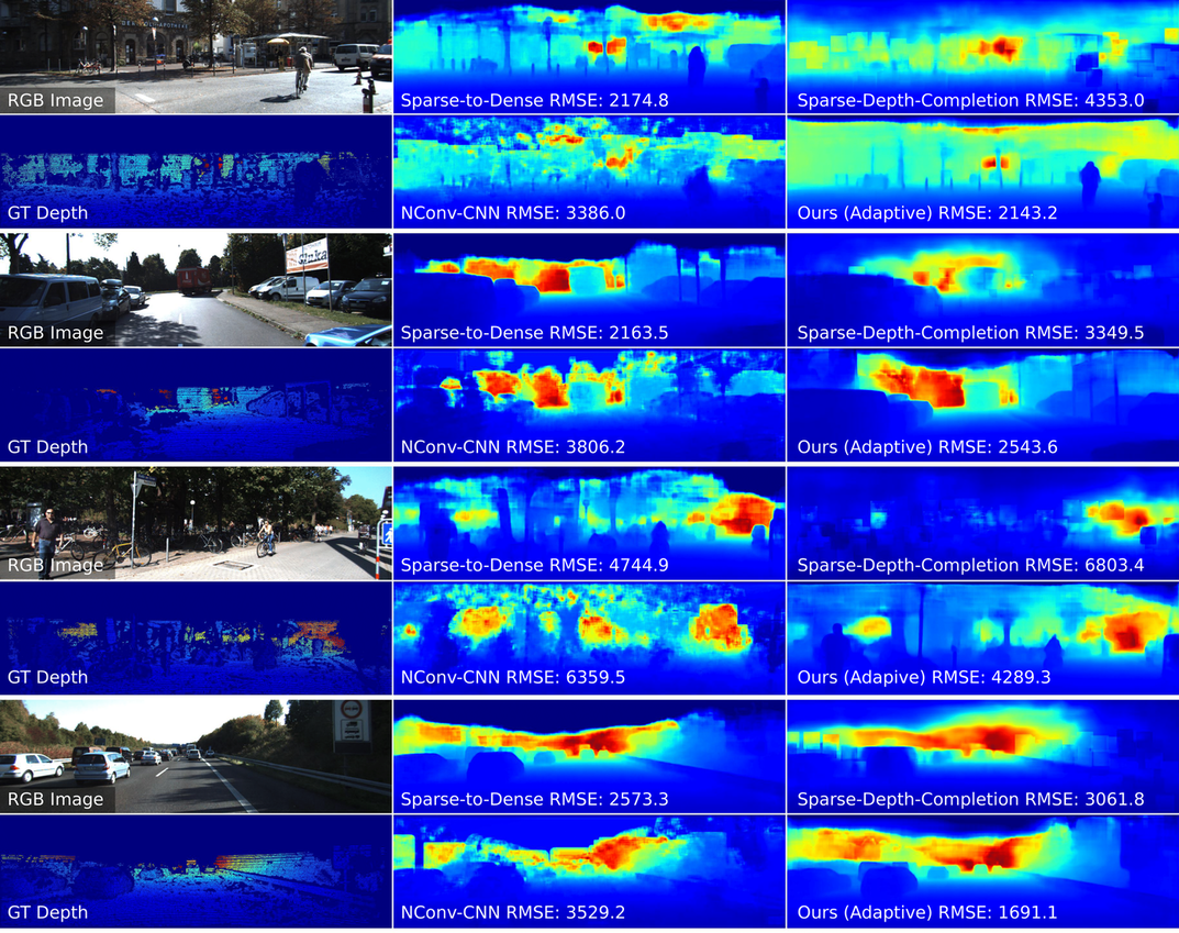
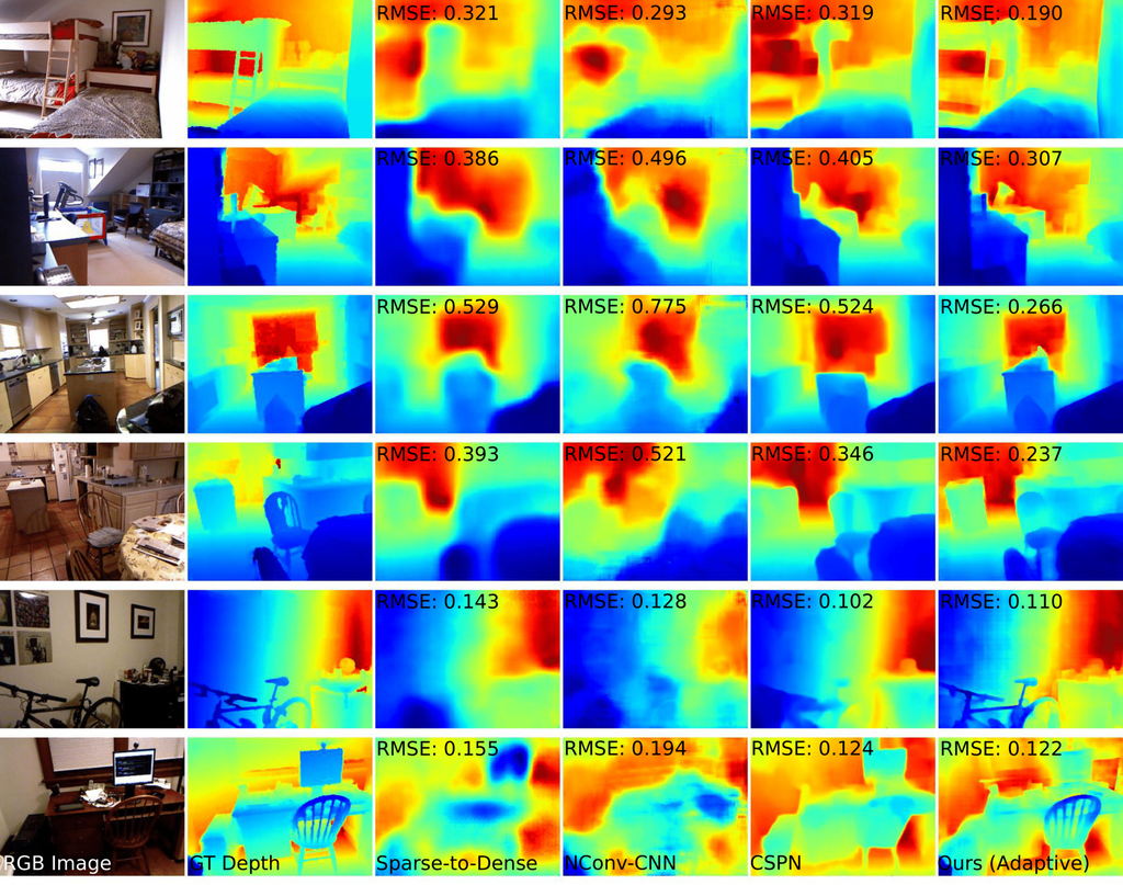
Depth completion results: (Top) Depth completion examples with RMSE (m) from the NYU-Depth-v2 dataset with comparisons to state-of-the-art depth completion methods. These results were obtained with an average of 50 samples per image. (Bottom) Depth completion examples with RMSE (mm) from the KITTI dataset with comparisons to state-of-the-art depth completion methods. These results were obtained with an average of 156 samples per image. Even when our method is out-performed, our reconstructed depth images still capture high frequency depth features with more accuracy.

Acknowledgments

A.W.B. and D.B.L. are supported by a Stanford Graduate Fellowship in Science and Engineering. This project was supported by a Terman Faculty Fellowship, a Sloan Fellowship, a NSF CAREER Award (IIS 1553333), the DARPA REVEAL program, the ARO (ECASE-Army Award W911NF19-1-0120), and by the KAUST Office of Sponsored Research through the Visual Computing Center CCF grant.

Citation

@inproceedings{Bergman:2020:DeepLiDAR,
author={Alexander W. Bergman and David B. Lindell and Gordon Wetzstein},
journal={Proc. IEEE ICCP},
title={{Deep Adaptive {LiDAR}: End-to-end Optimization of Sampling and Depth Completion at Low Sampling Rates}},
year={2020},
}